

Introduction
Materials and methods
1. Data collection
2. Statistical analysis
Results and discussions
1. Data verification
2. Derive linear regression
3. Regression verification
4. Discussions
Conclusions
Appendix
Introduction
In recent years, the livestock industry has experienced a significant increase in odor emissions due to the development of large-scale intensive farms (Post et al., 2020; Rappert et al., 2005; Van der Heyden et al., 2015). As a result, research on odor management and treatment technologies from livestock farms has been actively conducted (Wang et al., 2021). Odors from livestock farms contain hundreds of compounds, among which NH3 gas, H2S, volatile fatty acids (VFAs), and p-cresol are detected in various livestock farms (Wang et al., 2021). NH3 is the most common odor compound in livestock farms (Hanajima et al., 2010). In particular, a country with a mix of urban and rural areas, odor prediction technologies are being used to control odors in livestock environments in South Korea (Yoon et al., 2021).
Examples of odor prediction technologies include low-cost monitoring sensors integrated with information technology (Li et al., 2020), predictive modeling of odor diffusion using machine learning (Mulrow et al., 2020), and electronic nose technology that mimics the human sense of smell. Electronic nose (E-nose) systems have recently emerged as a technology for assessing livestock odors, and quantitative validation studies have been conducted. E-nose is an alternative technology that offers the advantages of quantitative analysis, fast measurement, high sensitivity and reproducibility, and objective odor identification without bias. An e-nose system was proposed for odor management in poultry farms, and its reproducibility was confirmed, showing a high correlation between odor and NH3 (Aunsa-Ard et al., 2021). Some studies have conducted VOC (Volitile Organic Compounds) concentration verification using e-nose and suggested that it is an effective method for detecting and categorizing volatile gases in livestock farms (Weng et al., 2021). In addition, H2S, which is mainly generated in livestock farms, was monitored, and modeled to analyze the degree of diffusion to control the concentration of H2S in ppb (Akter et al., 2020). However, the e-nose system is expensive and complex, so management is required (Van der Sar, I.G. et al., 2021). In Korea, information and communications technology (ICT) machinery, measured by odor sensors, is being distributed to manage livestock odors (Yoon et al., 2021).
The modeling for odor monitoring has been extensively studied. Modeling with data collected from water reclamation facilities around the city, such as H2S and weather sensors, yields an accuracy of more than 60% (Murlow et al., 2020). As complaints from landfill odors have become serious, CO2, NH3, H2S, etc. were measured around landfills to derive correlation analysis and prediction models (Du et al., 2023). Studies have also analyzed the correlation between odors and various environments. VOCs from vegetable proteins have been shown to increase in proportion to temperature, leading to higher odors during soybean spoilage due to high temperatures (Fischer et al., 2022). In addition, it has been shown that environmental variables such as temperature are correlated with the growth of aromatic substances and microorganisms in the vinegar fermentation process (Ruan et al., 2022). A study analyzing the correlation of fine dust and major odorants in pig farms found statistical significance between fine dust and H2S (Choi et al., 2022).
In this study, the co-relation between NH3 and meteorological data and prediction model for odor generation was derived by monitoring NH3 by attaching odor-measuring ICT equipment to eight farmhouses in an area with a high density of livestock in one region of Korea and analyzing the collected results.
Materials and methods
The experimental process is described as following. NH3, temperature, humidity, and rainfall were measured using real-time ICT. NH3 data have a difference in the number of raw data of each sensor owing to sensor failure and repair. The raw data were classified into farm/sensor/date using Excel and sorted in a time series by sensor for analysis. The analysis was performed monthly, excluding outliers in temperature, humidity, and NH3 concentration. Pearson's coefficient and VIF were calculated among the collected data to confirm the validity of the data. Subjects with high similarity were selected, and monthly regression equations were derived. Linear correlations between each factor were analyzed using Pearson’s coefficient analysis between NH3, temperature, humidity, and rainfall for each farm, and the independence between factors was judged by VIF. As a result of Pearson's correlation analysis, the detection point at each farm and period with the highest correlation were selected, and multivariate analysis (multiple linear regression model) models from NH3 with each weather data point were derived. Then, the models were verified with temperature, humidity, and NH3 data under the same environmental conditions as the monthly regression equation using R² and Mean Absolute Percentage Error (MAPE). The derived monthly NH3 regression equation was verified using R2 and MAPE analyses based on monthly meteorological data, excluding the corresponding month. Statistical software (SPSS 22.0, SPSS Inc., Chicago, IL, USA) was used for data analysis.
1. Data collection
(1) Target farms for data collected
The target area of this study was 8 livestock farms in Samseong-myeon, Eumseong-gun, South Korea. The farms were pig houses, and each farm was divided into piglet pens, sow pens, and finishing pig pens. A management system for monitoring livestock odor was attached to eight farms, and the NH3 concentration in each farm was collected. Table 1 presents the general status of the eight farms.
Table 1.
Results of general information about farms.
(2) Livestock Odor Monitoring System
The livestock odor monitoring system divided into ‘Livestock Odor Management System (LOMS)’ and ‘Livestock Odor Control System (LOCS)’. The LOMS is an ICT equipment for measuring livestock odors and consists of NH3 detection sensors that can measure the NH3 concentration. The NH3 concentration measured by the sensor unit was transmitted to the server through a communication device installed in the ICT. The LOCS is a system that can implement and monitor the data transmitted to the server and is composed of a server where the data are stored and a program that can be managed in real time (Yoon et al., 2021). The NH3 concentration measured using the sensor of the LOMS was implemented in the LOCS, and the data for each farm were extracted and used for analysis.
The NH3 measurement sensor was an electrochemical sensor MIX8415 (Mixsen, China). The measurement range was 0-100 ppm, and the error range is limited to within 5%. The test gas conditions were performed at 20 ± 2 ° C and 65 ± 5% RH, and the baseline range is -4 ppm to 4 ppm. As a result of operating the electrochemical sensor used in ICT equipment, the life expectancy is about 2 years and the calibration period is to be performed every 6 months. When calibrating the sensor, the user prepares a gas meter, standard gas (25, 50, 100 ppm), gas pressure regulator and calibration cap, and then supplies DC 24V, and connects the injection cap before gas injection. The zero point of sensor cannot be calibrated by injecting the standard gas in the atmospheric state, but also each standard concentration is injected for 3-5 min.
Two of ICT equipment installed at each livestock farm site were voluntarily selected in two places among the inside of pigsty, the boundary of the farmhouse, and the entrance to the manure treatment plant. Table 2 lists the sensor locations for each farm. NH3 data were collected for 6 months from September 2021 to February 2022.
Table 2.
Status of ICT sensors by 8 farms(2021.9 ~ 2022.2).
(3)Weather data (Temperature, humidity, and rainfall)
To detect the climate impact on each farm, a weather station measuring temperature, humidity, and rainfall was attached to each farm and measured. The weather station used for data collection was a WatchDog 2700 (Spectrum Tech, Inc., Aurora, IL), and installed at 3.0 m from the roof using a tripod.
2. Statistical analysis
(1) Data validation
The Pearson's coefficient is a numerical value quantifying the linear correlation between two variables (x, y). The Pearson correlation was calculated using the Cauchy-Schwarz inequality, and the calculation formula is Eq. 1. The estimated value has a distribution of from -1 to +1, and the closer to +1, the more positive linear correlation. Zero indicates no linear correlation, and a value closer to -1 means a negative linear correlation. Simply, it means that from -1 to -0.7 is a strong negative linear relationship, -0.7 to -0.3 is a moderate negative linear relationship, -0.3 to -0.1 is a weak negative linear relationship, -0.1 to 0.1 is a nearly negligible linear relationship, 0.1 to 0.3 is a weak positive linear relationship, 0.3 to 0.7 is a moderate positive linear relationship, and 0.7 to 1 is a strong positive linear relationship. Pearson's coefficient was used to analyze the linear correlation of time-series data (Xu et al., 2018) and the correlation between NH3 concentration and environmental conditions in farms (Yubo et al., 2021). In addition, the correlation between seasonal NH3 production in pig houses, environmental conditions, and pig weight was analyzed using Pearson's coefficient (Feng et al., 2022).
The VIF is a factor that can determine multicollinearity. In regression analysis, when the explanatory variables are highly correlated, the determinant of the variance- covariance matrix can be close to zero, resulting in very poor estimation precision of the regression coefficients, a phenomenon known as multicollinearity. A VIF value of 10 or more indicates multicollinearity, which means that an individual variable may not be able to act as a single independent variable and may be problematic for the results, so the variable should be dropped from the model (Chatterjee et al., 1991; Robert, 2011). The formula for calculating the VIF is (Eq. 2).
: R2 statistic from the regression of Xi on the other covariates
(2) Derive linear regressions
Using VIF and Pearson's coefficient, data with a high linear relationship were first screened to select farms A, B, C and H and from September 21 to December 21 to derive regression equations. NH3 concentration was selected as the dependent variable and temperature and humidity as the independent variables. Multiple regression analysis is a statistical technique for analyzing the degree of influence of independent variables on the dependent variable when there are two or more continuous dependent and independent variables (Mishra et al., 2010).
(3) Regression verification
R2 measures the accuracy of data prediction by calculating the variance of the predicted value relative to the variance of the actual observed value. It is distributed from 0 to 1, the closer it is to 1, and the higher is the explanatory ability of the equation. R2 is widely used to prove the explanatory ability of predictive and actual models (Shmueli et al., 2011). The equation for calculating R2 is given (Eq. 3).
Xpre,i: Prediction value
Xobs,i: observed value
The MAPE is used to test the similarity between the predicted model and the actual model, and the smaller the result, the more accurate the predicted model (Liu et al., 2022). If the result is greater than 50, the forecast is inaccurate; 20 to 50, reasonable forecasting; 10 to 20 good forecasting; and less than 10, highly accurate forecasting (Lewis, 1982).
n’: Total number of datasets used for estimation
Xpre,i: Predicted value of i-th sample
Xobs,i: True value of i-th sample
Monthly temperature and humidity ranges were applied to the derived regression equation to extract the NH3 generation amount of monthly data for each farm. Subsequently, data verification was performed using R² and MAPE using NH3 from different months of the sensor for which the regression equation was derived.
Results and discussions
1. Data verification
(1) Pearson’s coefficient
Pearson correlation analysis was conducted to analyze the linear correlation between the dependent variable (NH3) and independent variables (temperature, humidity, rainfall). When analyzing the correlation between temperature and NH3 concentration, the results were following; three strong negative correlations, nine weak negative correlations, 35 negligible correlations, one weak positive correlation, and seven strong positive correlations. In monthly results, there were 13 strongly negative or positive correlation anomalies (-1.0 to -0.3, 0.3 to 1.0) in September, 14 in October, 8 in November, 5 in December, (for 2021) 8 in January, and 6 in February (for 2022).
The results of linear correlation between rainfall and NH3 were as follows; 12 weak negative correlations, 51 almost negligible correlations, 20 weak positive correlations, and 3 strong positive correlations of 86 total results. The temporal range was designated as September to December because the Pearson's coefficient was relatively high (Table 3). Although rainfall was initially considered as an independent variable, it was excluded from the final regression model. Pearson correlation analysis indicated that rainfall showed consistently weak or negligible correlations with ammonia concentration across most farms and months. Therefore, rainfall was not considered a significant explanatory variable for predicting ammonia emissions in this study.
Table 3.
Results of correlation analysis for i) NH3 concentration and temperature; ii) NH3 concentration and humidity and iii) NH3 concentration and rainfall at each farm (A to H) from September 2021 to February 2022.
| Farm | Location | Sep. 2021 | Oct. 2021 | Nov. 2021 | Dec. 2021 | Jan. 2022 | Feb. 2022 | |
| NH3 : Temp. | A | S.B.1 #1 | -0.572 | 0.119 | 0.043 | 0.086 | 0.097 | 0.037 |
| S.B. #2 | -0.637 | 0.351 | 0.043 | 0.013 | 0.069 | 0.11 | ||
| B | S.B. #1 | -0.738 | 0.058 | 0.04 | 0.027 | -0.069 | -0.172 | |
| S.B. #2 | -0.413 | 0.026 | -0.202 | 0.133 | 0.173 | 0.012 | ||
| C | S.B. #1 | -0.554 | 0.316 | -0.094 | 0.105 | 0.205 | 0.375 | |
| S.B. #2 | -0.579 | 0.239 | -0.029 | 0.208 | -0.258 | 0.172 | ||
| D | S.B.#1 | -0.244 | 0.433 | 0.217 | 0.107 | 0.145 | -0.139 | |
| S.B. #2 | -0.634 | 0.277 | -0.241 | 0.052 | 0.061 | -0.219 | ||
| E | S.B. #1 | -0.465 | 0.116 | 0.051 | 0.086 | 0.37 | 0.12 | |
| M.T. 2 | -0.598 | 0.032 | 0.039 | 0.136 | 0.052 | 0.043 | ||
| F | V.O. 3 | -0.507 | 0.152 | 0.118 | 0.324 | -0.108 | 0.051 | |
| G | S.B. #1 | -0.579 | 0.24 | 0.01 | 0.272 | 0.199 | 0.153 | |
| V.O. | 0.025 | 0.406 | - | - | - | - | ||
| H | S.B. #1 | -0.717 | -0.019 | -0.11 | -0.019 | -0.097 | 0.05 | |
| V.O. | -0.727 | 0.067 | 0.029 | 0.247 | 0.057 | 0.07 | ||
| NH3 : Humidity | A | S.B. #1 | 0.733 | 0.534 | 0.371 | 0.145 | 0.318 | 0.165 |
| S.B. #2 | 0.761 | 0.317 | 0.031 | -0.219 | 0.376 | 0.249 | ||
| B | S.B. #1 | 0.808 | 0.72 | 0.544 | 0.204 | 0.404 | 0.298 | |
| S.B. #2 | 0.596 | 0.357 | 0.235 | 0.586 | 0.222 | 0.075 | ||
| C | S.B. #1 | 0.726 | 0.479 | 0.188 | 0.227 | 0.428 | 0.323 | |
| S.B. #2 | 0.761 | 0.508 | 0.176 | -0.13 | 0.176 | 0.329 | ||
| D | S.B.#1 | 0.258 | 0.324 | 0.143 | 0.058 | 0.126 | -0.056 | |
| S.B. #2 | 0.652 | 0.484 | 0.584 | 0.708 | 0.377 | 0.495 | ||
| E | S.B. #1 | 0.532 | 0.373 | 0.339 | 0.005 | -0.396 | -0.01 | |
| M.T. | 0.725 | 0.562 | 0.467 | 0.152 | 0.216 | 0.362 | ||
| F | V.O. | 0.635 | 0.493 | 0.201 | 0.14 | 0.032 | 0.153 | |
| G | S.B. #1 | 0.783 | 0.599 | 0.54 | 0.496 | 0.154 | 0.278 | |
| V.O. | -0.043 | 0.186 | - | - | - | - | ||
| H | S.B. #1 | 0.839 | 0.77 | 0.66 | 0.557 | 0.628 | 0.432 | |
| V.O. | 0.833 | 0.772 | 0.636 | 0.65 | 0.366 | 0.394 | ||
| NH3 : Rainfall | A | S.B. #1 | 0.105 | -0.155 | -0.077 | 0.026 | 0.16 | -0.056 |
| S.B. #2 | 0.071 | -0.1 | -0.102 | -0.046 | -0.037 | -0.035 | ||
| B | S.B. #1 | 0.073 | -0.101 | 0.101 | 0.024 | 0.175 | 0.114 | |
| S.B. #2 | 0.077 | -0.07 | 0.086 | -0.031 | 0.249 | -0.025 | ||
| C | S.B. #1 | 0.006 | -0.077 | -0.099 | -0.05 | 0.159 | 0.114 | |
| S.B. #2 | 0.086 | -0.024 | -0.177 | 0.06 | -0.069 | 0.257 | ||
| D | S.B.#1 | -0.072 | 0.15 | -0.026 | 0.019 | 0.422 | -0.07 | |
| S.B. #2 | 0.005 | 0.021 | 0.165 | -0.268 | 0.243 | 0.088 | ||
| E | S.B. #1 | -0.029 | -0.1 | -0.007 | 0.008 | 0.098 | 0.077 | |
| M.T. | 0.124 | -0.152 | -0.073 | 0.05 | -0.014 | 0.063 | ||
| F | V.O. | 0.054 | -0.06 | -0.045 | 0.131 | 0.028 | -0.005 | |
| G | S.B. #1 | 0.117 | -0.098 | 0.043 | -0.028 | 0.233 | 0.131 | |
| V.O. | -0.069 | 0.271 | - | - | - | - | ||
| H | S.B. #1 | 0.017 | -0.145 | -0.116 | -0.11 | 0.396 | 0.271 | |
| V.O. | 0.069 | -0.109 | -0.047 | -0.054 | 0.419 | 0.101 |
(2) VIF
The monthly VIF data for each measurement point are listed in the table 4. For the four types selected through Pearson's coefficient analysis, the September and December data did not have overlapping temperature and humidity ranges, making VIF analysis impossible. The monthly data for each of the four sites were found to have a VIF of 10 or less, preventing multicollinearity issues in the statistical analysis. The spatial range was set as A-S.B.#2, B-S.B.#1, C-S.B.#2, and H-V.O. for the VIF analysis and regression equation derivation (Table 4).
Table 4.
Monthly VIF analysis results compared to month of baseline.
2. Derive linear regression
The following results are a first-order regression of the dependent variable, NH3 concentration, collected by environmental sensors in the field, on the independent variables, temperature, and humidity, collected by the weather station for each month (Table 5).
Table 5.
Derivation of linear regression.
3. Regression verification
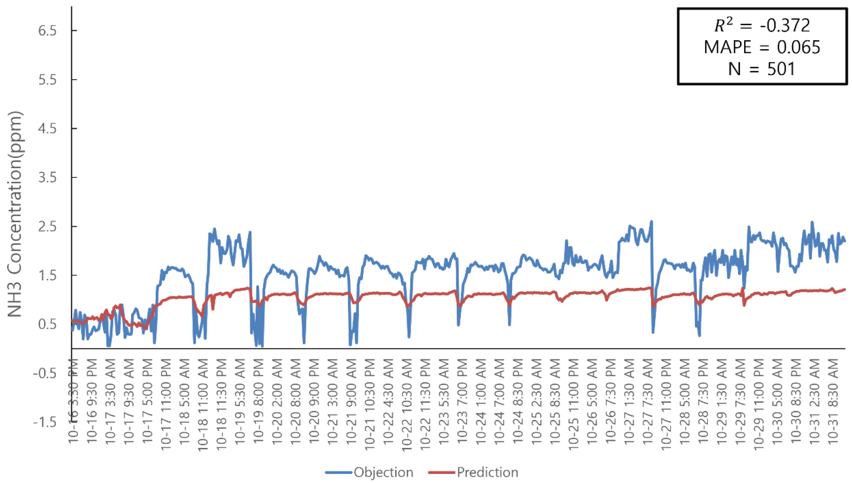
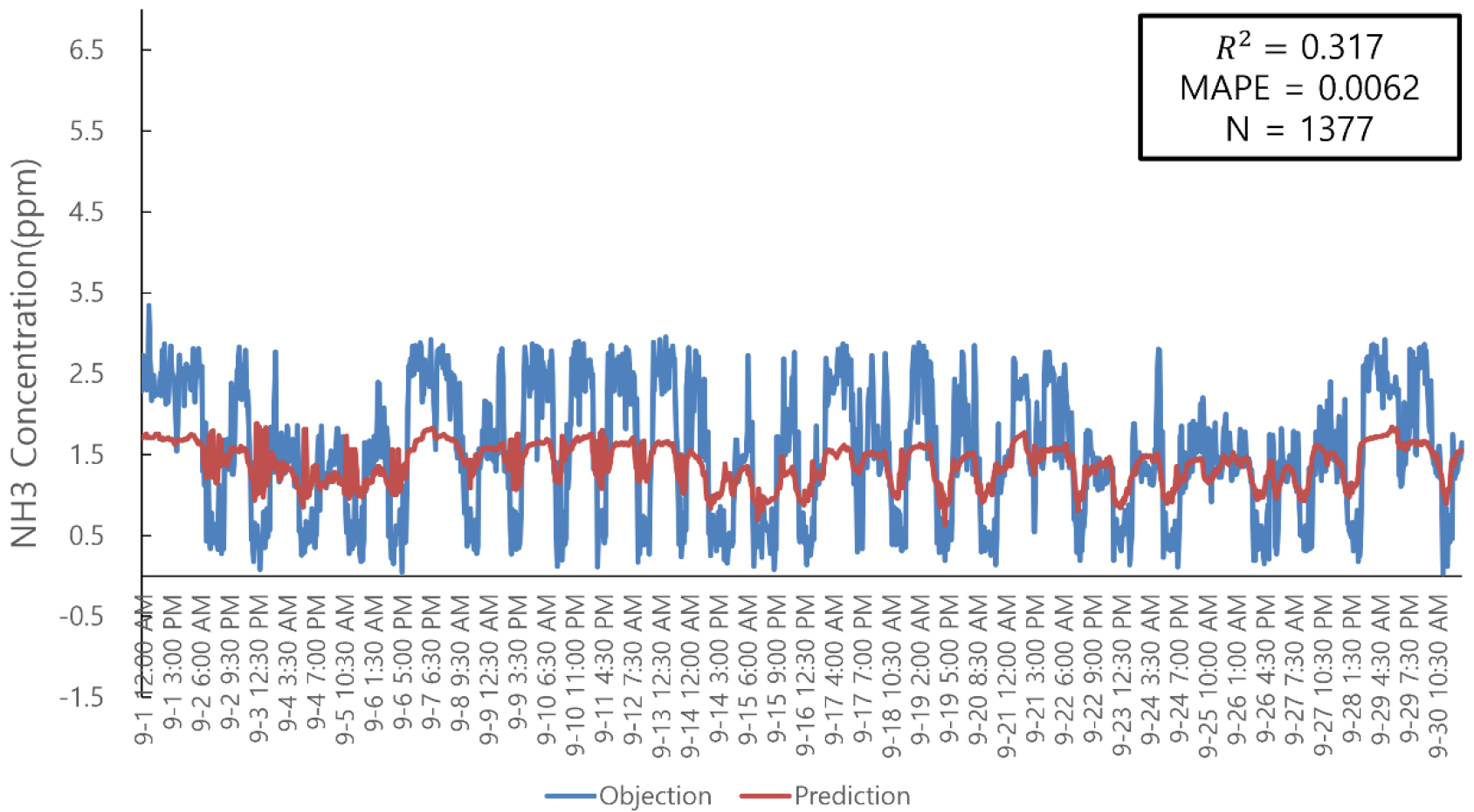
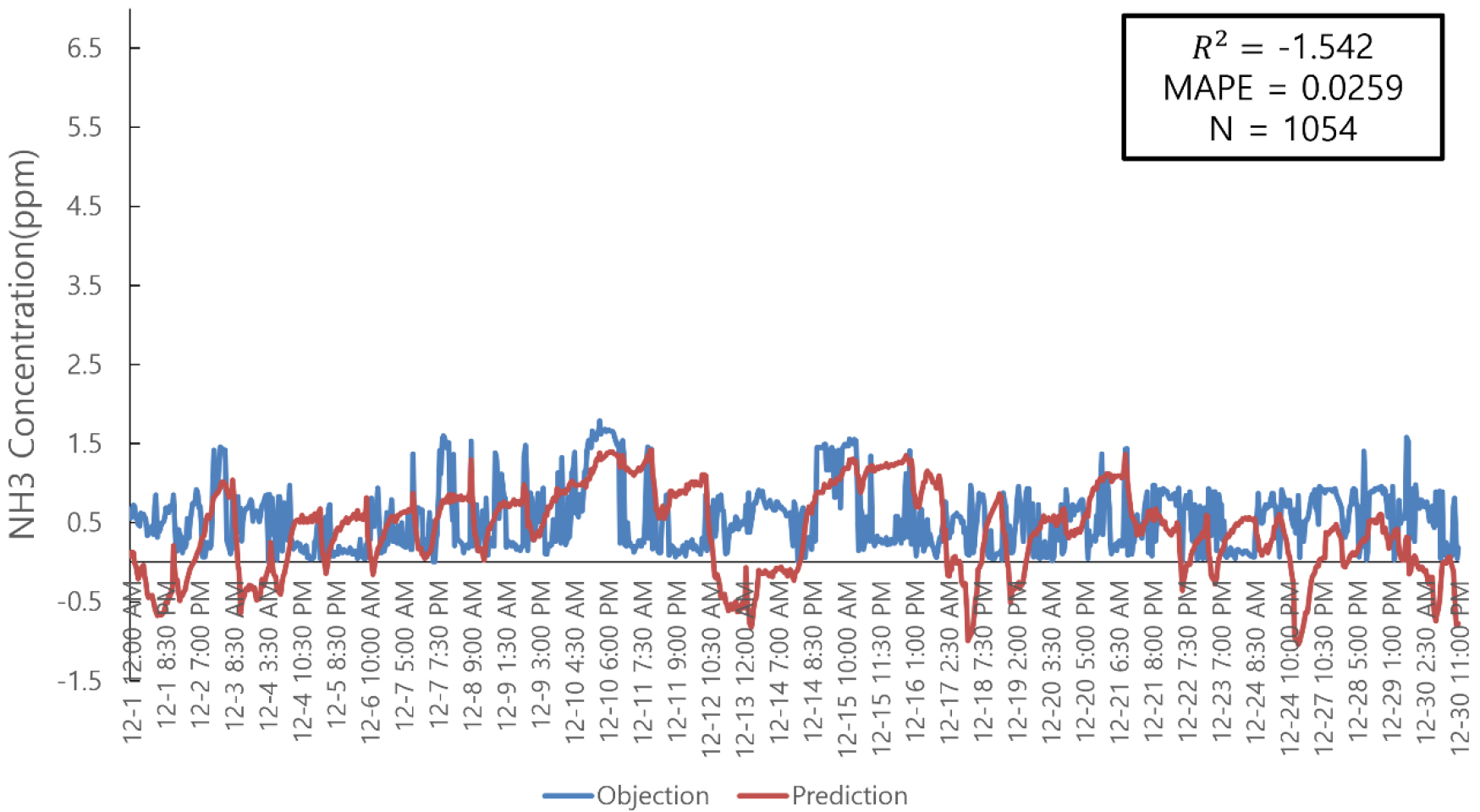
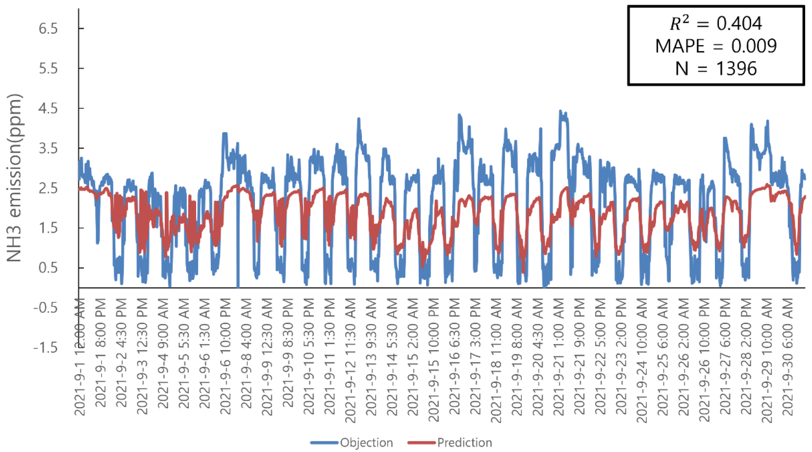
The following results show that R2 and MAPE are indicators of the accuracy of the predictive regression model. The data in September and December were excluded from the analysis for R² and MAPE because the temperature range measured by the temperature and humidity sensors was not high. In the MAPE results, all data were less than 10, indicating highly accurate forecasting. In particular, the relatively low magnitude of ammonia concentration values may have contributed to the low MAPE results, which should be carefully considered when interpreting prediction accuracy. However, in the R2 results, there were 13 results with significant values (R2>0.5, represented under the line of data) out of a total of 64, and the others were below 0.5 (Table 6). There were also R2 with negative values, so it is difficult to say that the estimated model is highly accurate. Figures 1, 2, 3, 4 show the graphs of high and low R2 among all data. These results suggest that it is difficult to predict the concentration of NH3 based only on environmental conditions (temperature and humidity), excluding external factors.
Table 6.
Results of R2 and MAPE at 4 points of sensor data.
4. Discussions
Various studies have been conducted on the factors affecting the spread of odors. Substances that affect livestock odor contained as NH3, H2S, VOC, etc., which can affect odor levels by binding to olfactory receptors due to their low molecular weight (Barth et al., 1984; Heaney et al., 2011; Huang et al., 2014; Pagans et al., 2006). Factors that directly affect the intensity of odor emitted from an odor source include the rate of release and diffusion of gases, atmospheric conditions (temperature, wind direction and atmospheric pressure) and topographical conditions (Barbusinski et al., 2021). These odorants are not proportional to the temperature or humidity (McCaul et al., 2021). Wind direction, wind speed, and atmospheric stability have been found to be important factors in the spread of odor (Conti et al., 2020).
Atmospheric particle modeling typically includes Gaussian, Lagrangian, and Eulerian methods. There are differences in each modeling method, but what they have in common is that they are mathematical models used to predict the concentrations of upwind air pollutants emitted from sources such as farms (Zhou et al., 2005). The Gaussian model simulates hourly average concentrations, as emissions and meteorological conditions can vary from hour to hour, and each hour's calculations are independent of those of the others (Danuso et al., 2015). The Lagrangian model is based on the idea that pollutant particles in the atmosphere move along trajectories determined by wind fields, buoyancy, and turbulence effects (Wilson et al., 1996). The Lagrangian model is very efficient, close to the source, and is particularly suitable for high point sources (Flesch et al., 1995). In the Eulerian (grid) model, the area under investigation was divided into grid cells in both the vertical and horizontal directions, and the average concentration of pollutant particles in each grid was calculated (Danuso et al., 2015). To predict the emission of particles into the atmosphere in three representative models, attention was paid to the meteorological state of the atmosphere, and the necessary meteorological factors were wind direction and wind speed.
Airborne particles from livestock operations, particularly those causing odor, include NH3, VOCs and particulate matter, PM10 and PM2.5 (Bibbiani et al., 2012). NH3 is an air pollutant that causes soil acidification, enrichment of nutrient nitrogen in ecosystems, and eutrophication of terrestrial and aquatic ecosystems. In air, it reacts with other compounds to form ammonium sulfate and ammonium nitrate aerosols, forming potentially hazardous secondary inorganic aerosols (PM2.5, Erisman et al., 2007; Kiesewette et al., 2014). The EU has identified the main key categories of NH3 emissions as: i) animal manure applied to land; ii) inorganic N-fertilizers; iii) non-dairy manure management; iv) cow manure management; v) pig manure management; collectively constitute 52% of total NH3 emissions (Wyer et al., 2022). Odor emissions from animal production facilities are composed of many variables, including animal species, housing type, feeding method, management factors, and manure storage and handling methods (Guo et al., 2004; Jacobson et al., 2005). Instead, the impact on nearby communities depends on the amount of odor emitted from the site, distance from the site, weather conditions, and topography, in addition to odor sensitivity and tolerance of neighbors (Danuso et al., 2015). Finally, the range of emissions depends on the size of the settlement, the stage of the rearing cycle, feeding operations, type of building, conditioning and ventilation, pavement and type of manure removal and collection system (Guo et al., 2006; Mielcarek et al., 2015).
Temperature and humidity, which are meteorological conditions, seem to correlate with odor emission concentrations in livestock farming, but they can be seen as independent factors. In this study, it was found that Pearson's coefficient, VIF analysis result, temperature, humidity result and NH3 emission concentration were significantly correlated, but the result of substituting actual measured data into the prediction equation built based on this result showed a very low correlation (R2, MAPE). It is noteworthy that the MAPE values obtained in this study were consistently below 10, indicating highly accurate forecasting according to conventional criteria. However, most of the R² values were low or even negative. This apparent contradiction arises from the different characteristics of the two evaluation metrics. MAPE reflects the average magnitude of prediction errors, whereas R² evaluates how well the model explains the variability and pattern of the observed data. In this study, NH3 concentrations often exhibited relatively narrow value ranges but irregular temporal fluctuations. As a result, the model was able to produce small absolute errors (low MAPE), while failing to accurately capture the variability pattern of the observed data, leading to low or negative R² values. This indicates that although the regression model may provide acceptable point-wise predictions under certain conditions, it has limited capability in explaining the underlying dynamics of NH3 emission patterns. This is thought to be a point to be aware of when performing odor reduction consulting for farmhouses or regions where many livestock odors occur.
In this study, the predictive performance of the regression models varied significantly among farms. In particular, Farm H showed relatively higher Pearson correlation coefficients (-0.717 to 0.839) and comparatively stable R² values (up to 0.65), whereas Farms A and B exhibited unstable results with several negative R² values. This discrepancy can be attributed to differences in farm-specific characteristics, including manure management systems, odor treatment facilities, and operational practices. As shown in Table 1, farms differ in terms of the presence of slurry pits, wet scrubbers, microbial supply devices, and liquid manure circulation systems. These factors are likely to influence NH3 generation patterns independently of meteorological conditions. Therefore, the results suggest that meteorological variables such as temperature and humidity alone may provide reasonable predictive performance only under relatively stable farm conditions. In contrast, in farms where NH3 emissions are strongly affected by internal operational variability, such as manure handling and treatment processes, the predictive accuracy of weather-based models becomes significantly limited.
This study has several limitations regarding the applicability of the derived regression models. First, the data were collected from a single geographic area (Samseong-myeon, Eumseong-gun), which may not represent other regions with different climatic and operational conditions. Second, the analysis was conducted on swine farms only, and therefore may not be directly applicable to other livestock species. Third, the regression equations were derived based on a limited temporal range (September to December), which does not account for seasonal variability throughout the entire year. Accordingly, caution should be exercised when applying the proposed models to different regions, livestock types, or seasons without additional validation.
Previous studies have identified wind speed, wind direction, and atmospheric stability as critical factors influencing odor dispersion and pollutant transport (Conti et al., 2020; Danuso et al., 2015). These variables play a key role in determining the spatial distribution and dilution of NH3 emissions. In this study, only temperature and humidity were considered as meteorological variables, which may explain the limited explanatory power of the regression models. It is expected that incorporating wind-related variables would improve model performance by better representing atmospheric transport processes. Future studies should therefore include wind speed and wind direction to enhance the predictive accuracy and applicability of NH3 emission models. These findings highlight that evaluation of predictive models for livestock odor should consider both absolute error metrics and variability-based indicators to avoid misinterpretation of model performance.
Conclusions
In this study, we aimed to determine the causal relationship between the environmental conditions (temperature, humidity, and rainfall) and NH3 concentration.
Correlation analysis was performed by measuring NH3, temperature, humidity, and rainfall for 8 similar farms, but the correlation was not high on the Table 3 (|R2|≥0.7, 15 of 132). In fact, it was not easy to apply the predictive regression equation because the environmental factors (temperature, humidity, rainfall) selected in this paper were not highly correlated with the odor generated by livestock farms. In addition, it was found that it was difficult to apply the predicted value of the regression equation even if the correlation was high under certain conditions. NH3 concentration cannot be determined causally only by temperature and humidity, but it is also necessary to comprehensively consider the farmers’ manure treatment method, pig management method, and odor treatment method.
In this study, a quantitative measurement method of factors reflecting the breeding characteristics of these livestock farms could not be prepared. However, if the correlation with NH3 concentration is analyzed by measuring factors such as odor diffusion, such as farm manager's behavioral pattern, wind direction, and wind speed, a methodology that can predict the odor derived from livestock farms can be developed. Future predictive models should incorporate wind-related variables and consider both absolute and variability-based evaluation metrics to improve accuracy and interpretation.
